ClearMap 2: Mapping activity with CellMap
ClearMap 2 is a powerful tool for performing whole-brain analysis, but if you are new to Python, or unfamiliar with troubleshooting tools developed in Python, you will likely run into trouble getting it to work straight out of the box. This series of guides were created to help you get started, from setting up a new Linux workstation for running ClearMap, to going through how to modify the scripts so that you have a useful foundation for performing your own analysis in ClearMap.
After following our previous post, you should have a working installation of ClearMap 2 ready to analyze whole brain data. The steps below will cover alignment and cell detection as well as performing group statistics. For a detailed walkthrough of the CellMap pipeline, including considerations for imaging samples for analysis, see our workshop recording.
Using and modifying the CellMap script to analyze cells
With the ClearMap environment active, we can use Spyder to edit and run the ClearMap scripts. Spyder can be opened simply by typing “spyder” in the active terminal window.
For this walkthrough, we will be modifying the example CellMap script available in the ClearMap directory (ClearMap\Scripts\CellMap.py). We also provide working scripts here.
1. Initializing the workspace and importing raw data from the light sheet microscope
Launch Spyder and open the CellMap.py script. You should see something similar to below:

In Spyder, you can run parts of a script (referred to as “cells”) by using Shift-Enter. If you try to run this cell you may encounter your first error - “No module named ‘ClearMap’ - to avoid this, you can specify where ClearMap is installed by including two lines at the top of this cell:
import sys
sys.path.append('/home/luke/Documents/Github/ClearMap2')
When importing raw data, the “directory” should be the folder containing subfolders with autofluorescence and cFos images. In our case, we are using example data from the original ClearMap paper. I’ve included the updated directory lines below to help with troubleshooting:
directory = '/home/luke/Desktop/Saline/1273'
expression_raw = 'cfos/15-42-19_0_8X-cfos_UltraII_C00_xyz-Table Z<Z,4>.ome.tif'
expression_auto = 'autofl/16-43-28_0_8X-autofluo_UltraII_C00_xyz-Table Z<Z,4>.ome.tif'
It’s also important to disable the debug mode. We can use this later for testing cell detection, but for now update to:
ws.debug = False
Now try running this cell again. The Console should list the files in the workspace and should include the raw and autofluorescence datasets (see image below). If these are listed as “no file” doublecheck the directories and filenames for spelling mistakes.
2. Initializing the alignment
The next cell is used to slice and orient the Annotation and Template/Reference files to match the volume of the dataset acquired at the light sheet microscope.

Annotation dataset: Intensity in this dataset is used to identify the different regions of the Allen Brain Atlas.

Template dataset: This dataset was created by imaging tissue autofluorescence using serial two photon tomography. A total of 1,675 brains were imaged to create this population based average.
Slicing can be performed on each axis (X, Y, and Z) and in the example provided only slices 1 to 255 (0, 256) of the annotation/template datasets will be used. In ClearMap the template brain is oriented such that the X axis = Dorsal-Ventral(DV), the Y-axis = Anterior-Posterior(AP), and the Z-axis = Medial-Lateral(ML). This means that slices 1 to 255 will be isolating roughly one hemisphere. It’s important to slice the template as close as possible to your dataset, as too large or too small a template volume will result in poor alignment and reduce the accuracy of cell localizations.
In addition to slicing, the orientation of the annotation/template dataset can be altered. If your experiment dataset matches the current orientation of the annotation/template then orientation should be (1, 2, 3). Use a - to flip the axis, and reorder these numbers to change axes. For example, if the dataset consisted of coronal sections like those in the images above, the orientation would be set to (3, 1, 2), with the AP or Z axis last.
Finally, the alignment parameters files are used by Elastix to perform registration. The provided files should work well with datasets captured on the light sheet microscope.
In this example, we are using the CellMap script to analyze the original single hemisphere CellMap datasets. For best results you should update this cell as below:
annotation_file, reference_file, distance_file=ano.prepare_annotation_files(slicing=(slice(None),slice(None),slice(0,228)), orientation=(1,2,3),
overwrite=False, verbose=True);
3. Resampling the data
Next, it is necessary to resample the data. The autofluorescence and cFos channels need to be downsampled to the resolution of the atlas being used (in this case the 25µm ABA)

Here, it is important your “source_resolution” correctly reflects the resolution of your experiment dataset. This will depend on the objective used and any additional magnification. In the example ClearMap datasets both the autofluorescence and cFos datasets have an image pixel size of 4.065µm and a step size of 3µm.
It’s important to note that when acquiring data for ClearMap, it is not necessary to acquire the autofluorescence and cFos data with the same conditions. This creates an opportunity to can save time during acquisition. Capturing lower resolution data for autofluorescence while maintaining sufficient resolution for accurate detection of cFos positive cells.
4. Image alignment
Now the datasets have been resampled to the atlas resolution, the CellMap script can perform alignment using Elastix. No changes are needed for these cells to work correctly.
The first step is a quick affine registration to correct for any misalignment between the autofluorescence and cFos channels. This is followed by aligning the atlas template dataset with the autofluorescence channel. Using Elastix 4.8, this process takes a little over 10 minutes.
After aligning the datasets, it’s important to open both the resampled autofluorescence image and the template image that has been aligned to this image. These can be found as below:
Resampled autofluorescence: \BrainFolder\resampledautofluorescence.tif
Template aligned to autofluorescence: \BrainFolder\elastix_auto_to_reference\result.1.mhd
Merging these images in Fiji is a convenient way to confirm the accuracy of the alignment.
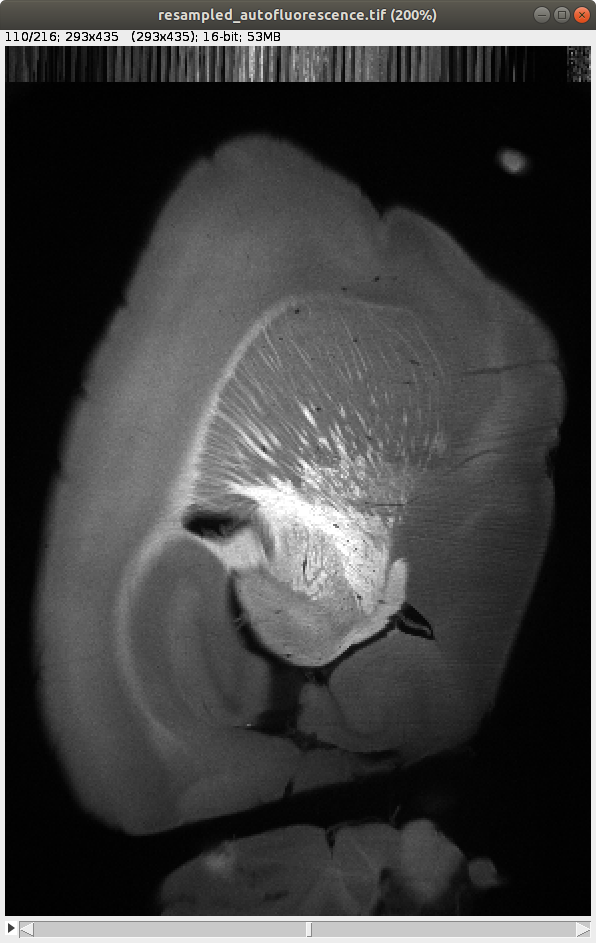
Raw data resampled to 25 x 25 x 25 µm

Template dataset aligned to raw data.

Merged channels. Looking for region edges and areas of contrast are useful for confirming alignment.
5. Preparing a sample dataset
A successful alignment will allow the locations of cells detected in the higher resolution cFos channel to be mapped into the atlas space, where we can use the annotation dataset to measure their intensity and determine the brain region they belong to.
A critical part of using CellMap is determining the best parameters for detecting cells. The script includes a useful cell for cropping out a small part of the experiment data for quickly testing and confirming cell analysis parameters. With ws.debug set to True, the cropped debug datasets will be saved separately with a “debug” suffix without changing the original complete dataset.

For the example ClearMap datasets, it is worth updating this cell to extract an area containing cells and the edge of the brain, to help optimize over a variety of cells (see below). For real experiments, a variety of regions and samples should be checked before confirming settings to be used for the project.
An easy way to find a region for cropping is to open the raw cFos dataset in Fiji. You can do this by dragging the folder containing cFos images onto Fiji, and checking on “Use Virtual Stack” - this allows you to view the entire dataset quickly, without needing to load the whole dataset into memory. With the image open, find a region you would like to crop. Then, while hovering over the top left and bottom right corner of this region, check the Fiji status bar - the image the coordinates listed here can be used for slicing in python.


Later, when you have finished testing parameters, comment out these lines and be sure to update ws.debug to False.
6. Cell detection parameters
The example script needs a few changes here to ensure successful detection on the original ClearMap example datasets. We share an updated script with working parameters here.
It’s important to include both a background subtraction step, as well as a threshold to exclude low intensities that are unlikely to be positive cells.
One of the advantages of the CellMap pipeline is making use of block processing to quickly analyze very large volumes. With a high-end workstation, you should be able to process a hemisphere in under 10 minutes. In our hands, using 128GB and 6 processes took 7 minutes.

7. Filtering detected cells
The detected cells can then be filtered further based on intensity (“source”) and size.

7. Cell alignment and annotation
The subsequent cells use Elastix to transform the cFos cell locations into the atlas space, so we can determine the brain regions they reside in. We recommend some changes here so that the final outputs include the region IDs and acronyms so that the CSV output tables are easier to explore and use outside of ClearMap for analysis and plotting.

8. Cell density/heatmap images
Finally, the script use the cFos cell coordinates transformed into the atlas space to create cell density images. In these images, each cell centroid is voxelized into a larger sphere with an intensity value of 1. As these spheres are overlayed and summed together the resulting image provides a way to visualize the cell density. These images are also useful for performing group statistics to locate areas of higher or lower cell density across groups
9. Performing group statistics and comparisons
To help you get started with performing group analysis in ClearMap2 we have included a script for creating mean and standard deviation images along with colored p-value images to find areas of comparatively higher/lower activation across groups.
We hope these scripts and notes are helpful in getting started using this great tool developed by Christoph Kirst and Nicolas Renier!